
Andreas Fichtner on the Frontiers of Seismic Imaging
Listen here or wherever you get your podcasts.

In the podcast, Andreas Fichtner describes the state of the art in seismic imaging. Despite enormous improvements in our capabilities over the past decades, there are still many structures and data types that remain elusive. Fichtner explains the various types of challenges faced by researchers seeking to sharpen our images of the Earth’s interior from seismic data. While some challenges appear insurmountable, others are gradually yielding to improved methods and computational power, and we can expect to see continual improvements over the next decade.
Fichtner is a Professor in the Department of Earth and Planetary Sciences at the Federal Institute of Technology in Zurich.
Podcast Illustrations
Images courtesy of Andreas Fichtner unless otherwise noted.
Numerical simulation of the L’Aquila earthquake of April 6, 2009
The numerical simulation shows surface waves that propagate along the Earth’s surface and body waves that propagate through the interior. In the podcast, Fichtner discusses the two types of body waves — primary (P) waves and secondary (S) waves. P-waves are longitudinal pressure waves, like sound waves, and S-waves are transverse shear waves. This simulation illustrates some of the paths taken by the seismic waves discussed in the podcast.

As Fichtner explained in the podcast, although the absolute size of the resolvable structures is much smaller in the case of medical ultrasound, the relative resolution of seismic images is better than that of ultrasound.
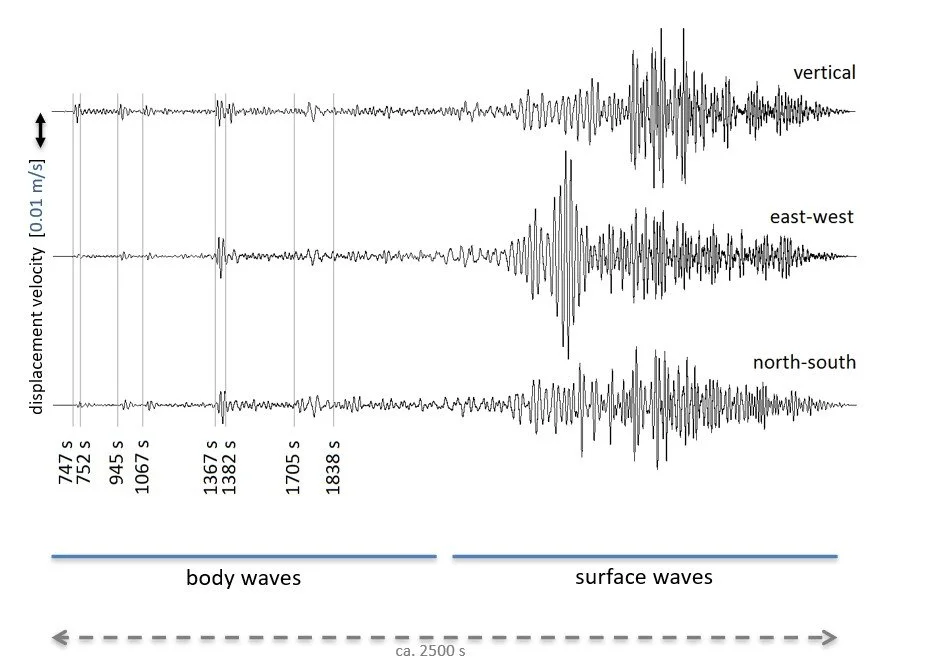
Seismic recording of S-waves (body waves) from the Tohoku earthquake that struck on March 11, 2011. The recording was made at the Black Forest Observatory in Germany, 83.3 degrees of latitude west of the earthquake epicenter. The body waves arrive first as they travel faster than the surface waves.
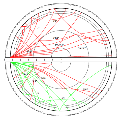
Each wave travels along a different path through the Earth and therefore “sees” a different part of the Earth. The diagram shows a section of the Earth with the simulated earthquake at left. The illustrative P-waves are shown in red and S-waves in green. The ray-path designations describe the wave type and its journey through different layers. P = primary wave; S = secondary wave; K = P-wave that travels through the earth’s outer core; c = reflection from the core-mantle boundary. Thus, for example, an ScP designation refers to an S-wave traveling toward the center of the Earth, reflecting off the outer core, and converting to a P-wave that travels upward. For illustrative purposes, S-waves propagating from the simulated earthquake are shown in the top hemisphere, and P-waves are shown in the bottom hemisphere (though some of them are then converted into S-waves).
Brian Kennett
Seismic Tomography Results from the REVEAL Model
REVEAL is a state-of-the-art 2024 model developed by Fichtner and his team. It incorporates by far the largest amount of data used so far in a single tomography. The model used about 460,072 graphics-processing-unit (GPU) hours, equivalent to about 52 GPU years using Cray XC50 compute nodes.
Thrastarson, S. et al. (2024) RVEAL: A Global Full-Waveform Inversion Model, Bulletin of the Seismological Society of America

Locations of the 2,366 earthquakes whose seismic waves were used in the model. The colors indicate how often an event was incorporated into an iteration, which ranges from 1 to 99. One of the factors used to determine the frequency with which an earthquake is included is how distinctive the earthquake is in relation to the others.
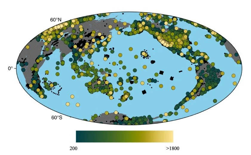
Locations of the 27,879 seismic stations used in the model. Colors indicate the number of earthquakes recorded by each receiver. Stations with fewer than 200 event recordings are shown as small black dots. The legend for the colored dots is shown by the bar below the map.
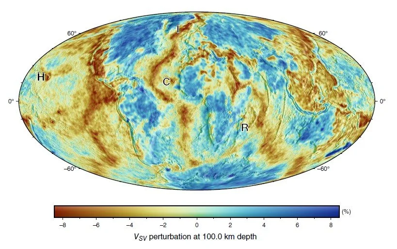
Horizontal slice at a depth of 100 km showing relative variations in the speed of vertically polarized S-waves (Vsv). The mid-oceanic ridges in the Atlantic and South Pacific show up prominently, as do hot-spot regions with active volcanism, such as Hawaii (H), Iceland (I), the Canaries (C), and La Réunion (R). The model also shows the contrast between the old, cold cratons and hot spots in Africa.

At a depth of around 200 km, subducting slabs come into sharper focus. The figure shows several of these, including the Nazca (N), Cocos (Co), and Caribbean (C) slabs, as well as the almost-continuous subduction of the Pacific plate (PP) beneath its neighboring plates toward Asia and Oceania.

The slice at a depth of 400 km reveals the subducting slabs that have advanced deeper into the mantle along the direction of subduction.

Close to the core-mantle boundary at 2,800 km depth, the slice shows the large-low-shear velocity provinces. These play an important role in our understanding of mantle dynamics and heat transport and are discussed in the podcast episode with Allen McNamara.
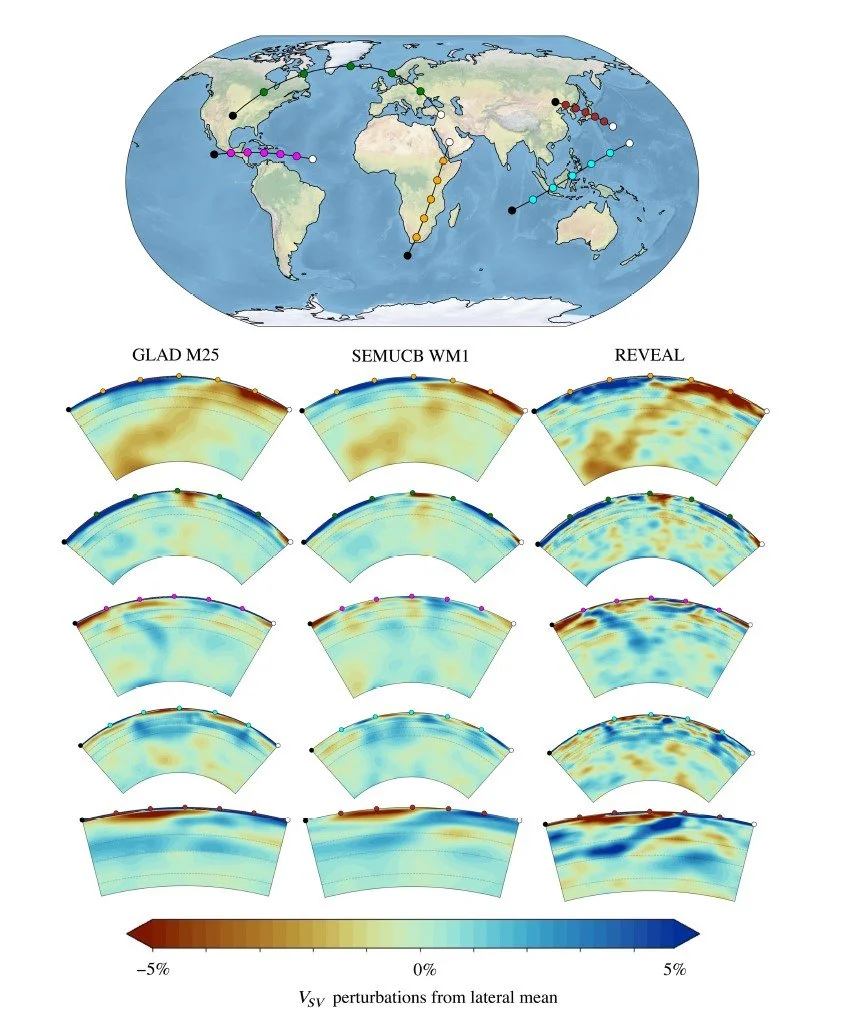
Comparison of cross sections of REVEAL with two earlier global tomographic models — GLAD M25 (Lei et al., 2020) and SEMUCB WM11 (French and Romanowicz, 2014). The geographical locations of the cross sections are indicated by the lines connecting colored dots on the globe, which correspond to the colored dots at the top of each section. The comparison shows how REVEAL produces sharper images, and hence cross sections than its predecessors. This enables us to place tighter spatial and temperature constraints on mantle features such as subducted slabs, the low-velocity region below east Africa, and (below) the Iceland plume.
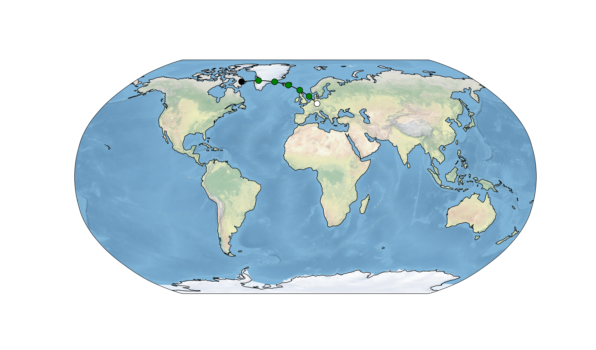
REVEAL cross section of Iceland plume. The location of cross section is shown on the map above, and the section down to the core-mantle boundary is shown at right. As Fichtner pointed out in the podcast, the Iceland plume is the only such structure that appears in all the tomographic models, while we have not yet been able to consistently image other suspected plumes, such as the one below Hawaii.

Using Fiber-Optic Cables as Seismometers
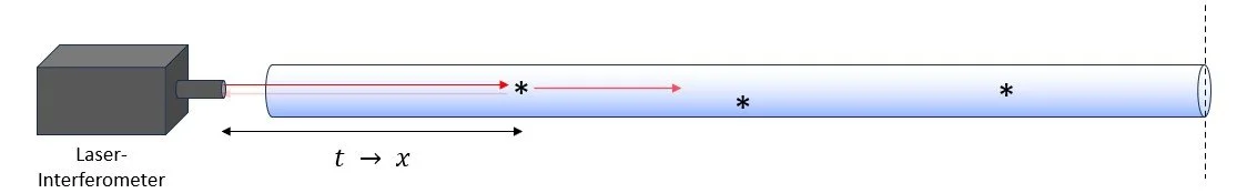
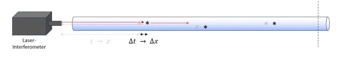
Fiber-optic cables include defects (*) that backscatter light passing along the cable. By measuring the round-trip travel time of light from the source to the defect and back using a laser interferometer, the distance to the defect can be calculated. When a seismic wave deforms the cable, there is a slight but detectable change in the travel time of the light to the defect, enabling the displacement caused by the seismic wave to be determined.
Applications of Fiber-Optic Seismic Sensing
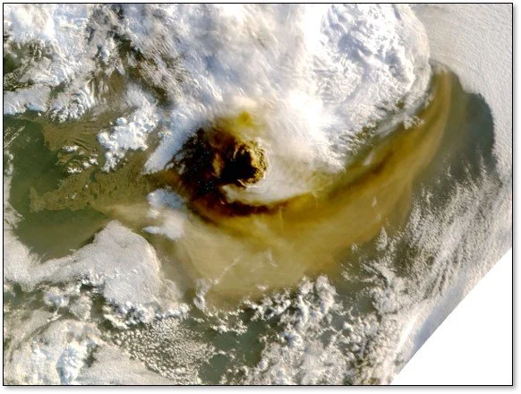
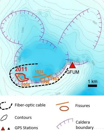
Fichtner and his team used a 12-km-long fiber-optic cable around and within the caldera to obtain high-resolution seismic data from Iceland’s most active volcano.
Monitoring Volcanic Earthquakes
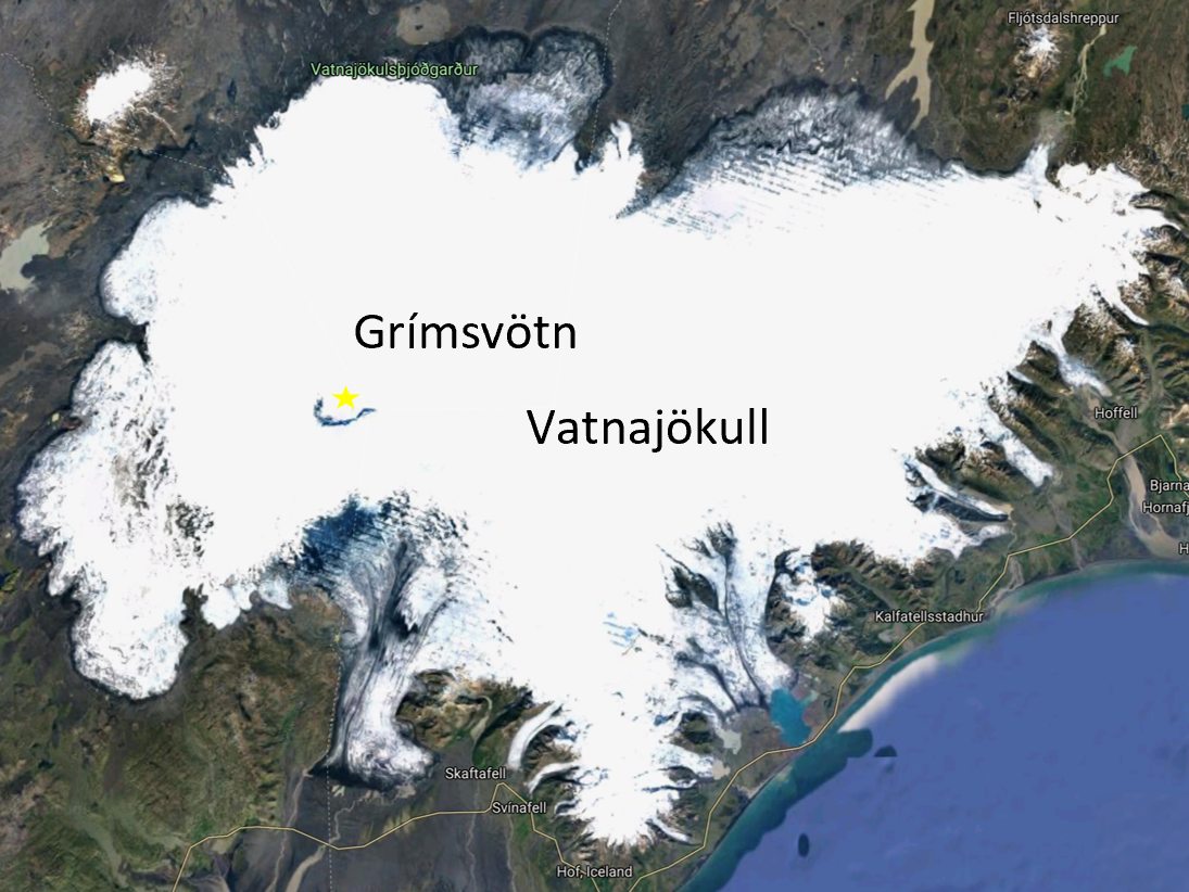

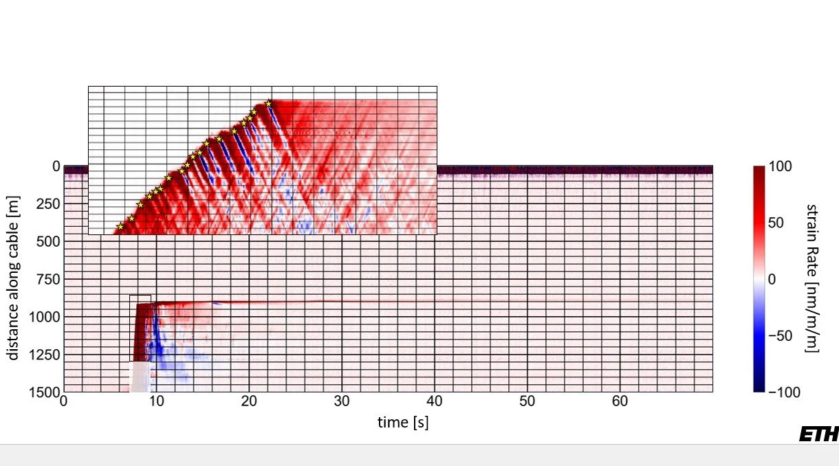
Fiber-optic data obtained during an eruption of Grimsvöten. This revealed about 1,000 small earthquakes a week, about 100 times more than the regional seismometer network was able to detect. This enabled the dynamics of the eruption to be monitored with much higher spatial resolution than was previously possible.
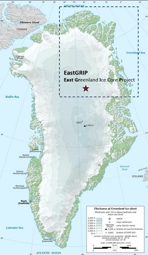
The Northeast Greenland Ice Stream is the largest ice flow in Greenland and transports 12 percent of Greenland’s ice flow to the sea. In the first experiment of its kind, Fichtner and his team laid a 1,500-m-long fiber-optic cable down a borehole in the ice. They then made a 14-hour continuous recording of the cable deformation. This revealed the presence of over 100 microquakes in less than a second.

Northeast Greenland Ice Stream

1,500-m-deep borehole in the ice.

Inserting the optic fiber into the borehole.
The results of Fichtner’s experiment show that hundreds of micro ice quakes occur within the space of a couple of seconds. The quakes are probably triggering each other in a kind of domino effect extending for hundreds of meters. It had previously been thought that such ice streams flowed like a viscous fluid. Instead, this experiment showed that they move in a rapid stick-slip motion.
Using Fiber-Optic Sensing to Image a Caldera
Biondi, e. et al. (2023), Science Advances 9, 42 DOI: 10.1126/sciadv.adi98

Map of the Long Valley Caldera, California study area showing the fiber-optic cables (green lines), seismic stations (blue triangles), and earthquakes (red dots). The black dashed line delineates the limit of the caldera.
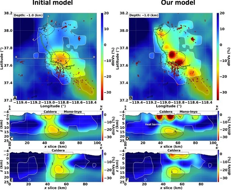
A fiber-optic cable was used to record earthquakes and seismic signals with much higher temporal and spatial resolution than was previously possible. Here, two fiber-optic cables covering an approximately 100-km north-south transect across the Long Valley Caldera in California. The panels on the left display S-wave anomalies from the initial model derived from the seismic-station data, while the panels on the right show the S-wave velocity anomalies obtained using the fiber-optic-cable data. The depth of the slices in the top panels is 1 km. The caldera and the extent of the lakes are shown by the black dashed lines. The panels in the 2nd and 3rd rows show model cross sections along the lines AA’ and BB’ indicated in the map shown above. The fiber-optic-based model shows a clear improvement in resolution as compared to the initial model.
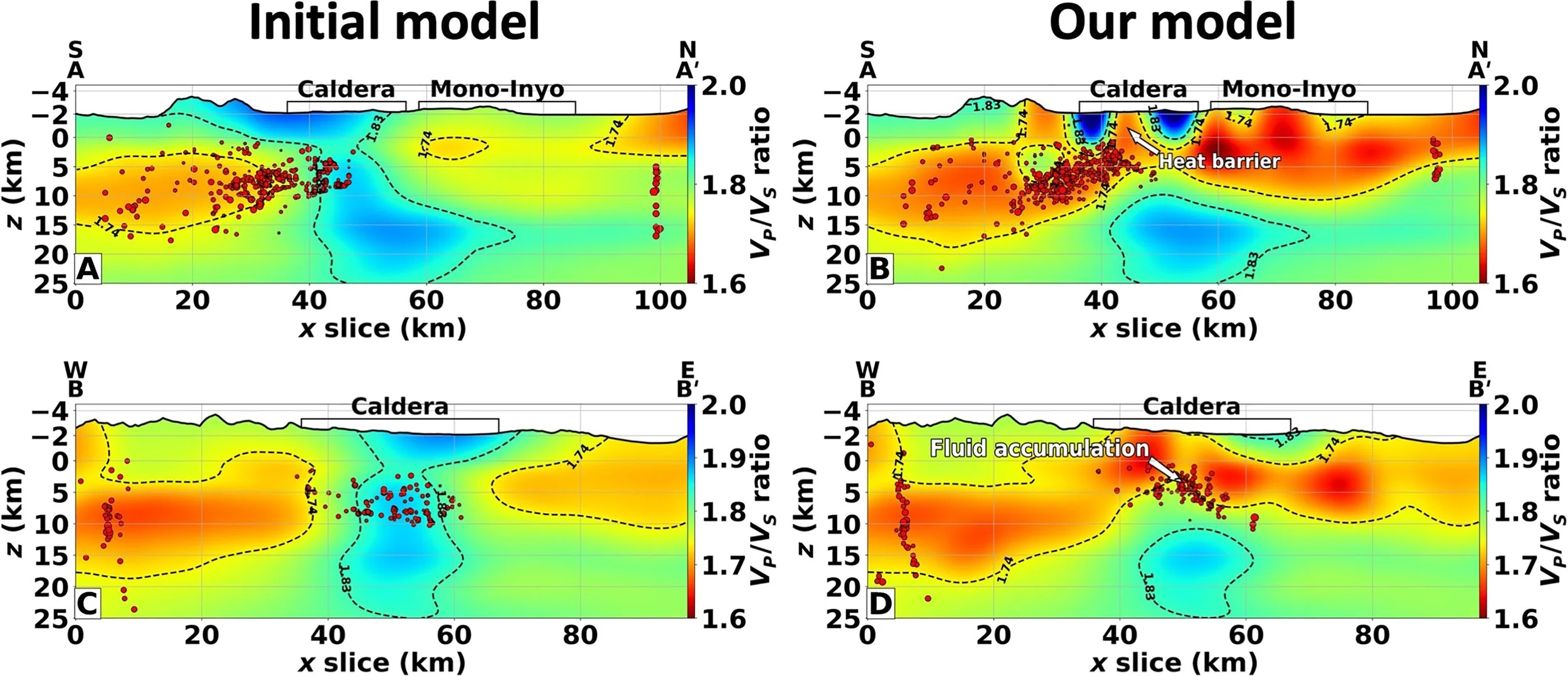
Sections showing the ratio of the P-wave velocities to the S-wave velocities along the sections AA’ and BB’ shown in the map above. The red dots indicate earthquakes occurring within 10 km of the cross sections. The fiber-optic-derived images highlight a definite separation between the shallow hydrothermal system and the large magma chamber located at ~12-kilometer depth. The combination of the geological evidence with these results enabled the researchers to determine the origin of the seismicity in the caldera. They concluded that fluids exsolved through second boiling provide the source of the observed uplift and seismicity.