
Isabel Montañez on the Late Paleozoic Ice Age as an Analog for Present-Day Climate
Listen here or wherever you get your podcasts
The late Paleozoic ice age began in the Late Devonian and ended in the Late Permian, occurring from 360 to 255 million years ago. It was similar to the present day in two key respects: rising atmospheric CO2 and recurrent major ice sheets. In the podcast, Isabel Montañez explains how we can use proxies to learn about the climate and ocean conditions that prevailed then. And with the help of a model, she says that we can also learn about sensitivities and feedbacks of Earth systems to rising CO2. Among other things, the model suggests that when the atmosphere reaches the present-day level of CO2, significant parts of the ocean may become anoxic and ocean circulation patterns alter.
Montañez is a Distinguished Professor in the Department of Earth and Planetary Sciences at the University of California, Davis.
Podcast Illustrations

Each of the 9 images above represents a proxy for CO2 in the geological past. A: Using the ratio of carbon-13 to carbon-12 isotopes in phytoplankton. B: Using boron isotopic ratios in foraminifera shells. C: Cuticle of Gingko biloba, which is the modern relative of the CO2 proxy plant group Ginkgoales in which the stomata density is a proxy for CO2. D: Diagram illustrating the inverse relationship between the density of stomata and atmospheric CO2. E: Diagram and equation for a mechanistic CO2 model that relates the concentration of atmospheric CO2 to the assimilation of CO2 during photosynthesis. F: Terrestrial plant proxies that use carbon isotope ratios measured in plant fossils or in sediments. Left: liverwort. Right: Medullosan frond. G: Using isotope ratios in the carbonates of paleosols. The image shows a calcite rhizolith (root cast) formed around a Permian tap root. H: Sample of bog iron from late Paleozoic soil, Argentina. The soil-formed iron oxide (goethite) it contains is used as the CO2 proxy. I: Thin-section photomicrograph of interlayered nahcolite (a sodium bicarbonate mineral) and halite. The nahcolite can be used as a CO2 proxy.
Using stomata as a proxy. Vascular plants optimize the number and size of stomata on their leaves to ensure sufficient CO2 uptake while minimizing water loss. Researchers can use the inverse relationship between frequency of stomata and CO2 to reconstruct paleo-CO2 concentrations.


Plots of oceanic depth vs. latitude of the time since a water mass has been in contact with the surface.
Younger ages in shades of purple indicate well-ventilated waters, whereas older ages in orange and yellow indicate poorly ventilated waters that typically correlate with low dissolved O2 in the deep ocean.
Together with the sea ice and mixing depth results, this suggests the onset of widespread seafloor anoxia during the CO2-forced warming despite being under deep glacial conditions.
Chen et al. 2002 PNAS

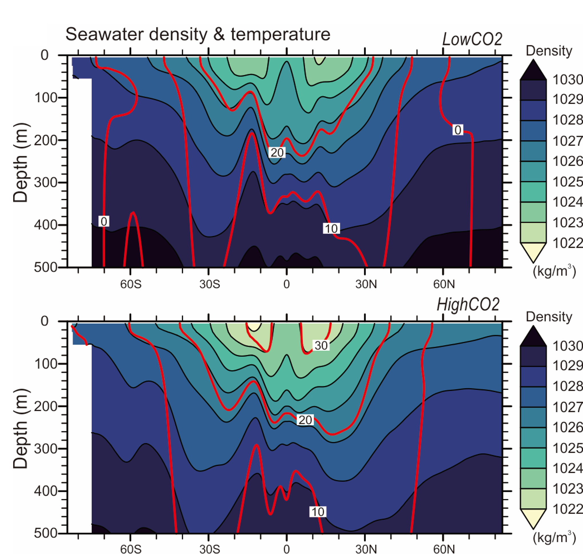
Simulations show the response of seawater density & temperature by depth for a doubling of CO2. Sea surface salinity (i.e., density) increases at low CO2 due to sea-ice formation, which excludes salt, thus creating briny water, whereas at high CO2 less sea-ice formation leads to decreased density overall.
Chen et al. 2002 PNAS
Results of the Earth-System Model for atmospheric CO2 levels of 280 parts per million (ppm) and 560 ppm for the late Paleozoic. Top row: sea ice forms at 280 ppm but not at 560 ppm. Bottom row: at 280 ppm, the late-winter mixed layer of the ocean is moderately deep but becomes much shallower at 560 ppm.
Chen et al. 2002 PNAS

Atmospheric CO2 levels during the late Paleozoic inferred from proxy measurements.
Montanez et al. 2016; Chen et al. 2022 PNAS